Roussel Guillaume1, Flores Olivier2
1. REUNIWATT, 14, rue de la Guadeloupe 97490 Sainte-Clotilde,
2. UMR PVBMT, 7 chemin de l’IRAT, 97410 Saint Pierre
1. Introduction
Cette étude est menée dans le cadre du projet DIVINES, dont les quatre objectifs principaux sont le déploiement d'outils de surveillance pour suivre les évolutions des écosystèmes de l'île, la production d'inventaires de biodiversité innovants, et enfin la fourniture d'indicateurs de biodiversité et de cartes de répartition à l'aide de SIG et des outils de télédétection. Nous nous intéressons ici à la capacité des données et méthodes de télédétection à améliorer la détection des plantes invasives. L'idée générale est d'évaluer la capacité des outils de télédétection à prendre en charge les techniques de cartographie au sol en étendant leur portée aux zones découvertes et aux horodatages. Deux approches ont été envisagées, une macroscopique et une microscopique. L'approche macroscopique vise à caractériser un taux d'invasion au niveau des pixels (Fenouillas et al., 2020) en utilisant une méthode de classification appliquée sur des jeux de données multispectrales. Parallèlement, l'approche microscopique est une approche orientée détection visant à cartographier la distribution d'abord et éventuellement la propagation d'espèces végétales spécifiques en utilisant des échantillons in situ géolocalisés comme données de référence (ONF, 2020). Notre travail a été mené sur la base de deux hypothèses principales. Le premier indique que lorsque l'on travaille avec des ensembles de données multispectrales, les informations spectrales ne sont pas suffisantes pour discriminer correctement les différentes espèces végétales. Cependant, la propagation d'espèces exotiques envahissantes devrait créer des motifs de texture distinctifs en relation avec la structure de la couronne et du feuillage d'une espèce particulière facilement reconnaissable grâce à la haute résolution spatiale de ces données. L'utilisation de caractéristiques texturales dans les processus de cartographie du taux d'invasion macroscopique et de détection d'espèces microscopiques devrait alors grandement améliorer la précision des résultats. Dans la suite, les deux approches seront abordées successivement, avec la présentation des données de travail et de référence, des caractéristiques texturales utilisées et des premiers résultats obtenus.
2. Approche macroscopique
2.1. Données de travail
Pour cette étude nous avons travaillé avec une acquisition SPOT extraite de la plateforme Kalideos, une base de données créée en 2001 par le CNES afin de valoriser les données de télédétection. L'image a été enregistrée le 7 juillet 2019, sur la partie sud-est de l'île de la Réunion, et nous avons considéré deux jeux de données, chacun associé à un niveau de traitement spécifique. Le premier est le niveau 1A (comptages numériques incluant l'étalonnage radiométrique et géométrique) que nous avons dû nous géoréférencer et le second est le niveau 2A, qui inclut l'orthorectification et les réflectances du sommet de la canopée. Nous nous sommes concentrés sur une partie spécifique du jeu de données correspondant à la zone du volcan et ses environs (cf. Figure 1).
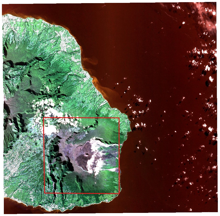
Figure 1: SPOT image (RGB) used in this study, with a specific focus on the area outlined in red
L'ensemble de données de vérité terrain utilisé afin de valider nos processus est une carte du niveau d'invasion global à l'échelle de l'île (Figure 2, Fenouillas et al, 2020). Cette carte est le produit de la combinaison de données d'enquêtes recueillies par plusieurs organismes (PNR, CBNM, ONF, DEAL) qui ont dû être harmonisées afin de constituer une carte de classification unique avec quatre classes de niveau d'invasion à 250 m de résolution horizontale : très faible /intact, faible, modéré et élevé.
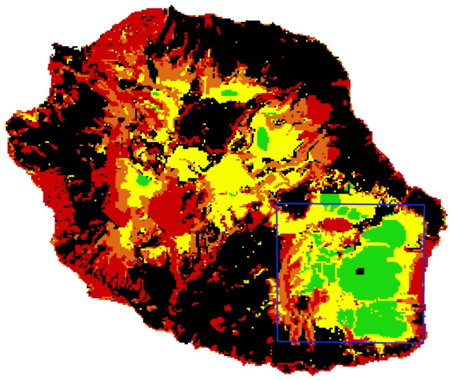
Figure 2: Invasion map characterized by four invasion levels (green : low / no invasion, orange : moderatly invaded, red: highly invaded, black: no data, Fenouillas et al. 2021)
Avant de commencer le processus de classification, tous ces jeux de données ont dû être co-enregistrés, y compris une étape de géolocalisation pour le jeu de données SPOT de niveau 1A et une étape de suréchantillonnage pour le jeu de données de validation afin qu'il puisse correspondre à la résolution spatiale de chaque jeu de données de travail.
2.2. Méthode de classement
L'objectif de cette étude est d'évaluer la capacité de l'information texturale à compenser la faible information spectrale fournie par les données multispectrales dans le contexte de la discrimination des espèces végétales indigènes/invasives. Notre cadre de classification est détaillé dans la figure 3.
2.2.1. Détermination des pixels de travail
Après l'étape de coregistration, un masque d'ombre est construit en utilisant l'espace colorimétrique c1c2c3 afin d'ignorer les pixels d'ombre. Cet espace colorimétrique est connu pour présenter de bonnes propriétés d'invariance des ombres (Salvador, 2004), et notamment la composante c3 :
$$c{3 = {tan}^{- 1}}(\frac{B}{\underset{❑}{max}{\{{R,G}\}}})$$
où , et sont respectivement les canaux rouge, vert et bleu de l'image SPOT. Le masque d'ombre est alors obtenu en seuillant cette nouvelle composante avec une valeur de seuil fixée à 0,95.
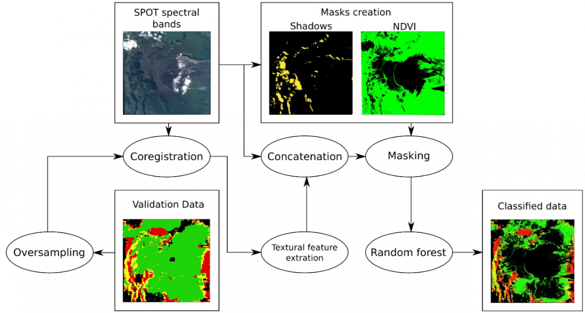
Figure 3: Chaîne de traitement pour la classification
Un masque de végétation est également construit afin de ne considérer que les pixels végétalisés. Ce masque est calculé en seuillant l'indice de végétation par différence normalisé (NDVI), calculé comme suit:
$$NDV{I = \frac{I{R - R}}{I{R + R}}}$$
où et sont respectivement les composantes infrarouge et rouge de l'image SPOT. Ici, nous considérons les pixels végétalisés comme ceux associés à une valeur NDVI supérieure à 0,2, ce qui correspond à différentes densités de végétation, de la très faible couverture de la canopée à la couverture complète de la canopée. Les pixels qui ne sont pas exclus par ces deux masques sont conservés comme pixels de travail dans notre étude. Les nuages sont associés à des valeurs de NDVI très faibles et seront donc exclus par cette étape de masquage ainsi que les pixels d'ombre et de non-végétation.
2.2.2. Extraction des caractéristiques texturales
En parallèle de l'étape de masquage, des caractéristiques texturales sont calculées à partir des quatre bandes spectrales de l'image SPOT. Dans cette étude, nous avons considéré deux caractéristiques différentes.
a. Haralick coefficients
Une matrice de cooccurrence (Haralick, 1973) est une structure de données présentant la proportion de pixels passant d'une valeur à une autre pour un décalage spatial donné, et un voisinage donné (Figure 4).
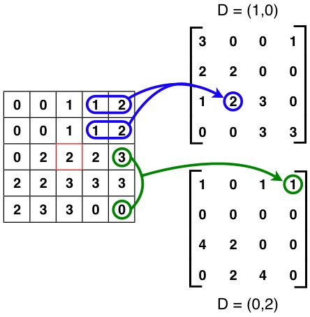
Figure 4 : Exemples de deux matrices de co-occurrence associés à deux déplacements différents (shift)
La taille de la matrice est égale au nombre de niveaux de gris dans l'image, il faut donc réduire la dynamique de l'image afin d'éviter la création de matrices gigantesques. C'est pourquoi les données étaient auparavant sous-échantillonnées dans une carte de classification de 16 classes en utilisant une version améliorée de l'algorithme K-means (Linde, 1980). Étant donné que les matrices de cooccurrence sont généralement grandes et clairsemées, diverses métriques sont dérivées de la matrice pour obtenir un ensemble de caractéristiques plus utile appelé coefficients de Haralick [9]. Ces coefficients sont liés à des caractéristiques texturales spécifiques de l'image (homogénéité, contraste, etc...) ou à la complexité et la nature des transitions de niveaux de gris qui se produisent dans l'image (cf. Figure 5).
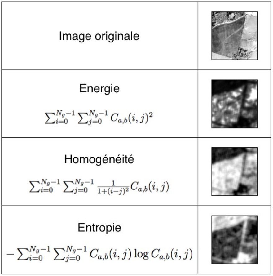
Figure 5 : Quelques exemples de coefficients Haralick à appliquer sur des matrices de co-occurrence
Dans cette étude, nous nous sommes concentrés sur quatre coefficients spécifiques : le contraste, l'homogénéité, l'énergie et la dissemblance. Ils sont calculés pour chaque pixel d'une bande spectrale à l'aide d'une fenêtre glissante, pour quatre décalages différents qui sont finalement moyennés : , , et . Enfin, cinq tailles de fenêtre sont considérées : 5, 10, 15, 20 et 25.
b. Profils morphologiques
Cette approche, initialement proposée par Pesaresi (2001), est basée sur des opérateurs de morphologie mathématique (Soille, 2003). Les profils morphologiques sont intrinsèquement liés au concept de granulométrie, qui vise à analyser la distribution statistique des tailles de structures dans une image en appliquant un ensemble d'opérations morphologiques associées à des éléments structurants (ie petite fenêtre de forme particulière caractérisant les voisinages sur lesquels l'opérateur est appliqué) de taille croissante, afin de construire des caractéristiques mettant en évidence des structures spatiales de plus en plus grandes à mesure que le quartier s'étend. Dans cette étude nous avons utilisé les mêmes opérateurs morphologiques que Fauvel (2008), à savoir l'ouverture et la fermeture par reconstruction. Ce sont des opérateurs géodésiques qui ne modifient pas les structures contrairement aux opérateurs d'ouverture/fermeture classiques mais n'enlèvent que celles qui sont plus petites que l'élément structurant. Dans un contexte non binaire, les profils d'ouverture mettront en évidence des structures sombres de taille croissante tandis que le profil de fermeture mettra en évidence des structures lumineuses de taille croissante (cf. Figure 6).

Figure 6 : Structure d'un profil morphologique étendu
Plusieurs tailles d'éléments structurants en forme de disque ont été testées pour construire les profils morphologiques étendus, de 4 à 68 pixels.
2.2.3. Algorithme de classification
A la fin du processus, les caractéristiques spectrales et/ou texturales que nous souhaitons utiliser pour construire la carte de classification sont concaténées, masquées et définies en entrée du classifieur, une implémentation Python de l'algorithme Random Forest fourni par la bibliothèque Sklearn . Il s'agit d'un algorithme supervisé, ce qui signifie qu'il doit être entraîné sur des données suffisamment exhaustives et représentatives afin de produire des sorties pertinentes. L'ensemble final de pixels valides est divisé en deux sous-ensembles : l'ensemble d'apprentissage (10 % des pixels valides) et l'ensemble de validation (90 % des pixels valides) sans chevauchement entre les deux. Le premier est utilisé pour produire un modèle qui est validé sur l'ensemble de validation.
2.3. Résultats et discussion
The whole testing area mentioned in part 2 is very large. In order to limit computing time for the following tests, we focused first on a smaller area (cf. Figure 7) and verified in the end that we are able to get approximately the same results on the large dataset with the most efficient set of parameters.
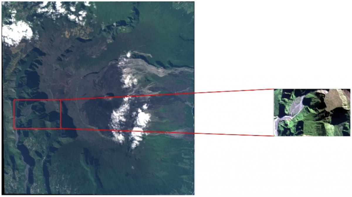
Figure 7 : Working area for the analysis of textural features parameters
The first series of tests were dedicated to spectral features only. Table I shows that multispectral information only is globally inadequate to evaluate the level of invasion. Whether with one spectral feature, the whole four or principal components (new features built through principal component analysis as linear combinations of the original features maximizing the variance of the dataset), the overall accuracy never exceed 60%. However we can already remark that the extreme levels of invasion (very low and high) are systematically better classified than the intermediate ones (low and moderate).
| Features | Classification accuracy (%) | ||||
| Very low | Low | Moderate | High | Total | |
| R | 46 | 41 | 34 | 34 | 39 |
| R + B | 60 | 46 | 33 | 54 | 49 |
| R + B + IR | 61 | 48 | 36 | 53 | 50 |
| R + G + B + IR | 65 | 54 | 41 | 68 | 57 |
| 4 PC | 69 | 54 | 44 | 70 | 59 |
Table I : Classification accuracies obtained with spectral features only. R = red, G = green, B = blue, IR = infrared and PC = principal component
| Features | Classification accuracy (%) | ||||
| Very low | Low | Moderate | High | Total | |
| MP [4, 8, 12] | 82 | 70 | 69 | 83 | 75 |
| MP [4, 20, 36, 52, 68] | 86 | 78 | 75 | 89 | 81 |
| HC [5, 10] | 76 | 63 | 65 | 77 | 69 |
| HC [5, 10, 15, 20, 25] | 91 | 79 | 85 | 88 | 85 |
| HC [5, 10, 15, 20, 25] | 92 | 87 | 92 | 89 |
Table II : Classification accuracies obtained with spectral and textural features. MP = morphological profiles (the numbers indicate the structuring elements used to built the profiles) and HC = Haralick coefficients (the numbers indicate the window size used to build the co-occurrence matrices)
With textural features concatenated to the spectral ones, the results are far better. Table II show that depending on the number of textural features given as input to the classifier, the results can be up to 30% more accurate than with spectral features only. It also shows that morphological profiles can quickly improve the accuracy of the classification even with a few small structuring elements but haralick coefficient computed with large windows lead in the end to better overall accuracies. The last line of the table finally shows that the fusion of the two intermediate classes is another way to improve the classification results, which means that these two classes are maybe too similar to each other.
All these results were obtained on level 1A SPOT data. Applied to level 2A SPOT data, results are systematically more accurate, with improvements ranging from two to seven percent compared to the less preprocessed data.
2. Microscopic approach
2.1 Données de travail
For this approach, we worked on the same SPOT 6 dataset than in the previous section, but we focused on three different sub-areas (cf. Figure 8). A reference dataset composed of several polygons corresponding to camphor trees (Cinamomum camphora, Lauraceae) and Cryptomerias (Cryptomeria japonica, Taxodiaceae), two species easily recognizable at canopy level, was provided by the Office National des Forêts (ONF). It is worth noting that only the camphor trees are considered as invasive. Cryptomerias are not but will be used as a second easily recognizable reference species.
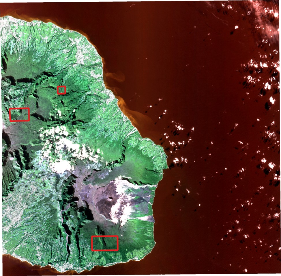
Figure 8 : SPOT dataset with the three new working sub-areas outlined in red
Each sub-area includes several polygons corresponding to planted sites of camphor trees and/or cryptomerias without shadow or cloud obstacles (cf. Figure 9).
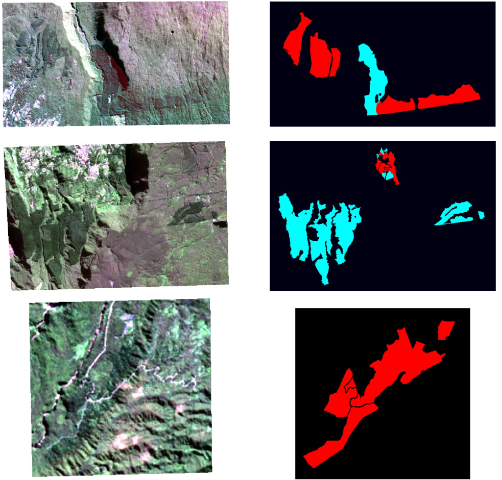
Figure 9 : The three areas of interest (SPOT data on the left, ground truth on the right), from area 1 on the top and area 3 on the bottom. Red polygons correspond to camphor habitats and cyan polygons to cryptomeria habitats (ONF, ??).
The number of samples for each species and each sub-area are listed in Table 3.
| Area 1 | Area 2 | Area 3 | |
| Camphor | 67132 | 4213 | 15926 |
| Cryptomeria | 23552 | 50410 | - |
Table 3: Number of samples for each species and each sub-area
3.2 Classification method and results
Several monoclass classification methods have been tested: One-class SVM, Isolation forests and Local Outlier Factor detection. These are supervised approaches for which 10% of the samples have been used for the learning step and 90% for the test step. One-class SVM produced by far the best results, so we will focus on this method only. Two quality criteria are considered:
- Precision (P) is the proportion of true positive (TP) samples over the whole number of positive samples, true and false (FP): P = TP / (TP + FP)
- Recall (R) is the proportion of true positive samples over the whole number of true samples: R = TP / (TP + TN)
The following tables show the results obtained with spectral features only (Table 4) and spectral/textural features (Tables 5 and 6).
| Area 1 | Area 2 | Area 3 | ||||
| P | R | P | R | P | R | |
| Camphor | 0.27 | 0.40 | 0.53 | 0.23 | 0.42 | 0.16 |
| Cryptomeria | 0.36 | 0.42 | 0.85 | 0.41 | - | - |
Table 4: Detection results obtained with spectral features only, with precision in red (P) and recall in green (R)
| Area 1 | Area 2 | Area 3 | |||||
| P | R | P | R | P | R | ||
| HC 5 | Camphor | 0.29 | 0.29 | 0.72 | 0.15 | 0.58 | 0.09 |
| Cryptomeria | 0.51 | 0.26 | 0.89 | 0.32 | - | - | |
| HC 5-15 | Camphor | 0.32 | 0.22 | 0.86 | 0.13 | 0.63 | 0.10 |
| Cryptomeria | 0.76 | 0.13 | 0.90 | 0.29 | - | - | |
| HC 5-15-25 | Camphor | 0.30 | 0.24 | 0.85 | 0.13 | 0.64 | 0.13 |
| Cryptomeria | 0.80 | 0.11 | 0.90 | 0.32 | - | - |
Tableau 5: Detection results obtained with spectral/textural features (Haralick coefficients), with precision in red (P) and recall in green (R)
| Area 1 | Area 2 | Area 3 | |||||
| P | R | P | R | P | R | ||
| MP 8 | Camphor | 0.58 | 0.19 | 0.56 | 0.23 | 0.83 | 0.08 |
| Cryptomeria | 0.68 | 0.24 | 0.93 | 0.25 | - | - | |
| MP 8-12 | Camphor | 0.70 | 0.18 | 0.53 | 0.21 | 0.86 | 0.06 |
| Cryptomeria | 0.66 | 0.24 | 0.95 | 0.22 | - | - | |
| MP 8-12-20 | Camphor | 0.71 | 0.18 | 0.54 | 0.22 | 0.77 | 0.07 |
| Cryptomeria | 0.73 | 0.25 | 0.96 | 0.23 | - | - | |
| MP 8-12-20-36 | Camphor | 0.71 | 0.18 | 0.44 | 0.22 | 0.77 | 0.10 |
| Cryptomeria | 0.73 | 0.26 | 0.96 | 0.24 | - | - | |
| MP 8-12-20-36-52 | Camphor | 0.65 | 0.21 | 0.51 | 0.23 | 0.65 | 0.10 |
| Cryptomeria | 0.73 | 0.29 | 0.96 | 0.25 | - | - |
Tableau 6: Detection results obtained with spectral/textural features (Morphological profiles), with precision in red (P) and recall in green (R).
Spectral only results are not very accurate, in terms of both precision and recall. The only exception concerns the cryptomeria on area 2 for which the detection precision is quite good (Table 4). Adding textural information to the detection process has various effects depending on the species, the area and the type of feature used. First, it must be noticed that the use of textural features systematically decreases recall rates by a factor of up to four, but overall increases precision, in particular for Camphor. Haralick coefficients greatly increase the precision of the detection of cryptomeria trees on area 1, but were nearly useless for the detection of camphor trees. On area 2, it is the exact opposite while on area 3, a slight improvement can be noticed for the detection precision of camphors. When these features are effective, they are all the more effective as the scale of the coefficient is high. Morphological profiles slightly increase the precision of the detection for all three areas and for both cryptomeria and camphors but this improvement does not grow with the scale of the textural feature (Table ). Sometimes, it even decreases.
We note however that the quality of the spatial data regarding the actual distribution of the focal species is relatively poor. Better results should be obtained with better resolved and more accurate field data.
4. Conclusion and perspectives
In this study, two approaches for the analysis of the spread of invasive vegetal species using remote sensing data were addressed. The first one is a classification framework using both spectral and textural information to discriminate several overall qualitative levels of alien plants invasion. We showed that in this context, the presence of textural information is crucial to produce relevant classification results. The second one is a detection method focused on detecting particular plant species. It aims at detecting a single known class among an unknown number of other classes using the very same spectral and spatial features as the first approach. Unfortunately, the results of this second approach are much less promising. Even if the textural information generally increases the precision of the detection algorithm, it comes at the price of a drastic decrease of recall. It means that the algorithm is less often wrong but also that the proportion of undetected valid samples is higher.
As perspectives, we have a few tasks in mind. The first one would be to test the generalization capacity of the Random Forest classification models created in this study over datasets acquired on different timestamps, especially for top of canopy data (level 2A). Secondly, we would like to test how much the phenology could improve the two approaches by building models based on several datasets acquired throughout the same year. A third possibility would be to investigate the potential of ITC (Individual Tree Crown) characterization methods on high-resolution data (Pléiades) and finally, to replace the One-class SVM used for the second approach by a convolutional neural network.
Références
Asner, G. P., Jones, M. O., Martin, R. E., Knapp, D. E., Hughes, R. F., 2008. Remote sensing of native and invasive species in Hawaiian forests. Remote Sensing of Environment, Volume 112, Issue 5, Pages 1912-1926.
Asner, G.P., Martin, R.E., Knapp, D.E., Kennedy-Bowdoin, T., 2010. Effects of Morella faya tree invasion on aboveground carbon storage in Hawaii. Biol. Invasions 12, 477–494.
Atkinson, J.T., Ismail, R., Robertson, M., 2014. Mapping bugweed (solanum mauritianum) infestations in pinus patula plantations using hyperspectral imagery and support vector machines. IEEE J. Sel. Top. Appl. Earth Obs. Remote Sens. 7 (1), 17–28.
Chang, H., Burke, A., 2014. Integration of hyperspectral and polarimetric radar remote sensing techniques for monitoring invasive weeds. 2014 IEEE Geoscience and Remote Sensing Symposium, Quebec City, QC, pp. 2950-2952.
Elton, C.S., 1958. The Ecology of Invasions by Animals and Plants. Methuen, London.
Espinar, J.L., Díaz-Delgado, R., Bravo-Utrera, M.A., Vilà, M., 2015. Linking Azolla filiculoides invasion to increased winter temperatures in the doñana marshland (Sw Spain). Aquat. Invasions 10, 17–24.
Fauvel, M., Benediktsson, J.A., Chanussot, J., Sveinsson, J.R., 2008. Spectral and spatial classification of hyperspectral data using svms and morphological profiles. IEEE Trans. , Int. Geosci. and Rem. Sens., vol. 46, n°11, pages 3804-3814.
Fenouillas, P., Ah-Peng C., Amy, E., Bracco, I., Dafreville S., Gosset, M., Ingrassia, F., Lavergne, C., Lequette, B., Notter, J.-C., Pausé, J.-M., Payet, G., Payet, N., Picot, F., Poungavanon, N., Strasberg, D., Thomas, H., Triolo, J., Turquet, V., Rouget, M., 2021. Quantifying invasion degree by alien plants species in Reunion Island, Austral Ecology
Gaertner, M., Den Breeyen, A., Hui, C., Richardson, D.M., 2009. Impacts of alien plant invasions on species richness in Mediterranean-type ecosystems: a meta-analysis. Prog. Phys. Geogr. 33 (3), 319–338.
Ghulam, A., Freeman, K., Bollen, A.,Ripperdan, R., Porton, I., 2011. Mapping invasive plant species in ropical rainforest using polarimetric Radarsat-2 and PALSAR data. 2011 IEEE International Geoscience and Remote Sensing Symposium, Vancouver, BC, pp. 3514-3517.
Hellmann, C., Große-Stoltenberg, A., Thiele, J., Oldeland, J., Werner, C., 2017. Heterogeneous environments shape invader impacts: integrating environmental, structural and functional effects by isoscapes and remote sensing. Sci. Rep. 7, 4118.
Hestir, E. L., Khanna, S., Andrew, M. E., Santos, M. J., Viers, J. H., Greenberg, J. A., Rajapakse, S. S., Ustin, S. L., 2008. Identification of invasive vegetation using hyperspectral remote sensing in the California Delta ecosystem. Remote Sensing of Environment, Volume 112, Issue 11, Pages 4034-4047.
Hughes, F. R., & Denslow, J. S. (2005). Invasion by a N2-fixing tree alters function and structure in wet lowland forests of Hawaii. Ecological Applications, 15, 1615−1628.
Lawrence, R. L., Wood, S. D., Sheley, R. L., 2006. Mapping invasive plants using hyperspectral imagery and Breiman Cutler classifications (randomForest). Remote Sensing of Environment, Volume 100, Issue 3, Pages 356-362.
Linde, Y., Buzo, A., Gray, R.M., 1980. An algorithm for vector quantizer design. IEEE Trans. Commun. Pages 84-95.
Lu, S., Shimizu, Y., Ishii, J., Washitani, I., Omasa, K., 2012. Detection of invasive plant with hyperspectral imagery in the riverbed of Kinu River, Japan. 2012 IEEE International Geoscience and Remote Sensing Symposium, Munich, pp. 4813-4816.
Matongera, T.N., Mutanga, O., Dube, T., Lottering, R.T., 2016. Detection and mapping of bracken fern weeds using multispectral remotely sensed data: a review of progress and challenges. Geocarto Int. 1–16.
ONF (Office National des Forêts), 2020. Carte des types de végétation, Version 1.2..
Peerbhay, K.Y., Mutanga, O., Ismail, R., 2015. Random forests unsupervised classification: the detection and mapping of solanum mauritianum infestations in plantation forestry using hyperspectral data. IEEE J. Sel. Top. Appl. Earth Obs. Remote Sens. 8 (6), 3107–3122.
Pejchar, L., Mooney, H.A., 2009. Invasive species, ecosystem services and human wellbeing. Trends Ecol. Evol. 24 (9), 497–504.
Pesaresi, M., Benediktsson, J.A., 2001. A new approach for the morphological segmentation of high-resolution satellite imagery. IEEE Transactions on Geoscience and Remote Sensing, 39(2), pages 309-320.
Royimani, L., Mutanga, O., Odindi, J. , Dube, T. , Matongera, T. N. , 2019. Advancements in satellite remote sensing for mapping and monitoring of alien invasive plant species (AIPs). Physics and Chemistry of the Earth, Parts A/B/C, Volume 112, Pages 237-245.
Salvador, E., Cavallaro, A., Ebrahimi, T., 2004. Cast shadow segmentation using invariant colour features. Computer Vision and Image Understanding, 95, pp. 238-259.
Shackleton, C., Shackleton, S., Buiten, E., Bird, N., 2007. The importance of dry woodlands and forests in rural livelihoods and poverty alleviation in South Africa. Forest Policy Econ 9 (5), 558–577.
Soille, P., Morphological Image Analysis, Principles and Applications. Germany : Springer-Verlag.
Somers, B., Asner, G. P., 2013. Invasive Species Mapping in Hawaiian Rainforests Using Multi-Temporal Hyperion Spaceborne Imaging Spectroscopy. in IEEE Journal of Selected Topics in Applied Earth Observations and Remote Sensing, vol. 6, no. 2, pp. 351-359.
Vaz, A. S., Alcaraz-Segura, D., Campos, J. C., Vicente, J. R., Honrado, J. P., 2018. Managing plant invasions through the lens of remote sensing: A review of progress and the way forward, Science of The Total Environment, Volume 642, Pages 1328-1339.
Zhang, L., Wang, M.-H., Hu, J., Ho, Y.-S., 2010. A review of published wetland research, 1991–2008: ecological engineering and ecosystem restoration. Ecol. Eng. 36, 973–980.